Variability in Traffic Emissions Using Simulation Models
Comments (0)
February 18th 2019
Cite
Birt, Andrew; Nunez, Cristhopher, 2019, "Variability in Traffic Emissions Using Simulation Models", CARTEEH DATA:HUB, http://carteehdata.org/library/document/variability-in-traffic-emissions-using-simulation-models (accessed Apr 24 2024)


Introduction
In the interest of understanding the relationships between emissions due to controlled traffic characteristics on a second by second instance, this paper presents the process of simulating, storing, generating emissions and the analyzation of the results. Traffic generated pollution is a common topic of interest for many researchers because of its importance to public health. We explored a smaller portion of emissions, in particular – vehicular emissions activity. The emissions generated on a road within a time period are random – and will depend on the number, types, and speed of vehicles passing within that time period. Since averages are not representative of true exposure, modeling the impact of emissions on people’s health through dispersion models becomes too theoretical and unrealistic.
This randomness may have important consequences for studying and assessing the impact of vehicle pollutants on human health. In this case, we are interested in the variability in emissions for two specific areas of traffic, a four-way junction and a two lane road. For each case, we ran 5 simulations where each simulation introduced a gradual increase in cars. Simultaneously, each simulation was analyzed for two exposure periods, 100 second and 500 seconds. To achieve this analysis, four tools were used to arrive at the our results; SUMO traffic simulator, Python, MySQL Database and R Studio. The results suggest that a probabilistic approach to modeling vehicle emissions and concentrations may be important for evaluating the impacts of traffic emissions on human health, especially when modeling or measuring near road concentrations.
SUMO
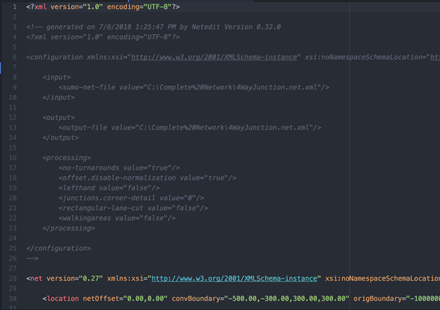
We began the process by using SUMO, a traffic simulator that allows the user to generate car emissions second by second. To begin using SUMO, a Windows, Linux or Mac OS computer is needed with either 32bit or 64bit capacity. Downloading the software is easy and is available for free on the website http://sumo.dlr.de/index.html . To achieve our desired outcomes, 2 graphic user interfaces were used: "netedit.exe" and "sumo-gui.exe.", "netedit.exe" was used to build our road network under the conditions we desired. The interface allows a user to build roads, junctions, control traffic with stop lights and many other parameters. The "netedit.exe" then saves the network as an XML file which will define the road the cars travel on.
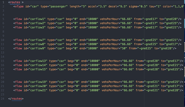
Next we defined the routes the cars would take in a file ending in .rou.xml as well as the amount of cars the road will sustain.
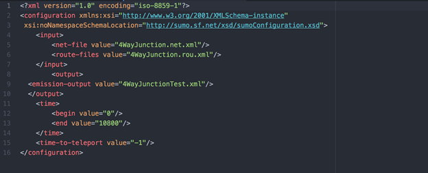
Finally we defined the configuration file ending in sumo.cfg that is used to visualize the simulation. Here we defined the inputs (the net file and route file) and defined the outputs (an emissions output file with second by second information). The user must open and run the simulation in the sumo-gui.exe window to generate the second by second information file. The output of the configuration file is the time separated information of all the cars in the desired simulation (a good practice is to keep all the data we use in a single file or directory so we avoid any errors in coding later).
Python
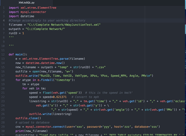
Because we wanted to extract the data into easy to read tables, we required the use of python to extract the XML file generated by the sumo configuration file. First in the MySQL database, we created an empty table where we would store all the necessary information. We then created this file to sort through each line separated by time, extract the information we wanted, stored it in a temporary CSV file, and then upload it directly into a MySQL database table we had pre made.
MySQL Database
Within the database, 16 tables (along with database settings) defined by MOVES (Motor Vehicle Emissions Simulator) were pre-loaded into the desired schema (the database we choose) for reference in our code in R studio. We also prepared an emissions table with all the desired sections to store the desired emissions information (position, time, speed, type of vehicle, operating mode). The tables in MySQL are cross referenced by the R Code that generates the emission we used to analyze the data.
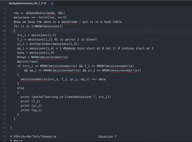
R Studio
A lot of computing power takes place in this section because of the amount of raw data that we process, lot of improvements could be made in this code, but it works great for our data. Here we used two pieces of code that first generate the emissions we needed and the second code outputs variance graphs and data results. A lot of the heavy lifting is done by SecbySecEmissions_CN_7_17.R file. Within this R-code, the data was queried to show each distinct vehicle, at each time step until it left the simulation grid. Knowing its basic information, MOVES uses VSP and STP equations to categorize cars into different operating modes. After converting all of the speeds and acceleration points from SUMO, MOVES then generates the emissions using the different tables from MySQL and equations that are provided in the R Code.
Within the second R-code, we then queried cumulative emissions from the MySQL data table “emissions” to generate cumulative emissions. Within that section, we then analyzed 100 seconds of exposure vs 500 seconds.. These graphs represent the visual range, and variability of cumulative emissions.
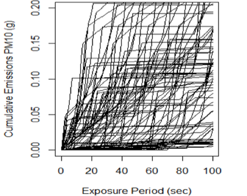
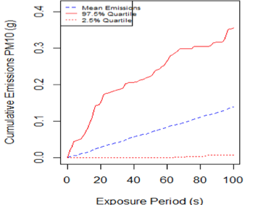
Each instance/line represents a single test subject measuring the cumulative mass of PM10 for the given time period. To remove any correlation from measuring emissions consecutively, we recorded emissions staggered by 20 seconds.
To get a full grasp of how the variability changes, we analysed 5 simulations with the following changes as well as the results in how variability changed with more exposure time, and with increasing car flows.
- Simulation Time= 10,800 seconds (3 hrs.), Vehicles per hour=400 (Veh/hr), Start time=300 seconds into simulation, Exposure period= 100, 500 seconds, Staggered by 20 seconds (RUN ID: 1)
- As 1 but increase Veh/hr by 10% (RUN ID: 2)
- As 1 but Increase Veh/hr by 20% (ID: 3)
- As 1 Increase Veh/hr by 50% (ID: 4)
- As 1 Increase Veh/hr by 100% (ID: 5)
These are the results we generated for the two traffic networks for the 5 simulations:
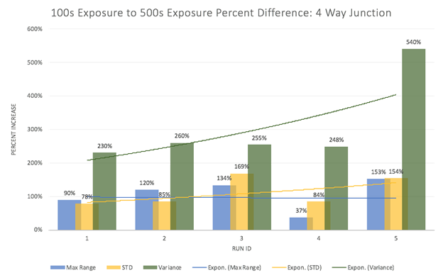
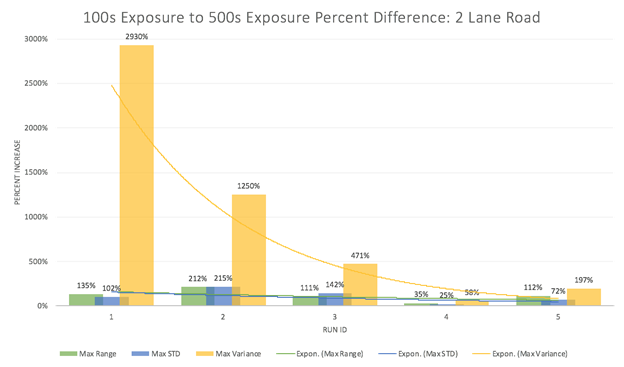
The traffic generated through SUMO and the emissions generated with MOVES allowed us to generalize the effects of exposure times. Higher exposure periods usually lead to higher variations in cumulative emissions, where in most cases, increasing car flow has no considerable effects. With these outcomes, we can think of areas with high stop and go traffic to have the most varied cumulative emission as exposure time increases. While areas of high speed and constant motion tend to have high variation with longer exposure with low car flows, but decrease as more cars added.
The methods used in this study can be used in a variety of studies by any researcher or anyone who is interested in the topic. The basic framework can be implemented in scenarios related to traffic modeling, emissions, pollutant exposure, and can enhance the accuracy of dispersion models, with few alterations to the source code. Implementing a dispersion model to generate second by second concentrations would be the next step towards a full chain model where traffic, emissions, dispersion, exposure and health impacts are evaluated simultaneously. This full chain model would allow researchers and others alike to trace and identify, health impacts, potential solutions and policy changes that can then further protect our environment as well as our quality of life
FILES (8)
-

4WayJunction.sumocfg.xml
Size: 824 Bytes
Last Modified: Sun Feb 17 2019This code is the product of defining the inputs and outputs of a SUMO simulation, running the simulation and then producing this file as an output. It must be saved as a .sumocfg file to run in the sumo gui.
-
4WayJunction.rou.xml
Size: 2 KB
Last Modified: Sun Feb 17 2019This code defines cars and the routes they will take while running through a SUMO simulation , this code must be used in conjunction with a .net.xml and .sumcfg file
-

SecbySecEmissions_CN_7_17.R
Size: 12 KB
Last Modified: Sun Feb 17 2019This code simply takes information from a MySQL Database through query, uploads the data into the R environment, uses MOVES created by the EPA to generate emissions rates for vehicles based on speed and acceleration second by second for all specified vehicles.
-

Create_SQL_table.sql
Size: 559 Bytes
Last Modified: Sun Feb 17 2019Creates a table for reference in MySQL Workbench 8.0
-
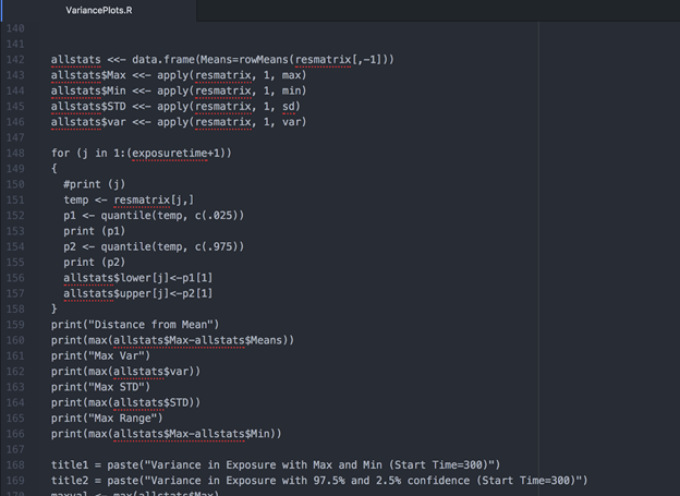
VariancePlots.R
Size: 5 KB
Last Modified: Sun Feb 17 2019This code takes information from a MySQL database that has time separated information on vehicle emissions, plots the cumulative emissions of a specified SUMO simulation area and outputs statistical information on the data.
-

XMLtoSQL.py
Size: 2 KB
Last Modified: Sun Feb 17 2019This code extracts data from a sumo XML file containing emissions data, stores it as a temporary csv file and then proceeds to store it in a pre defined MySQL data table.
-
4WayJunction.net.xml
Size: 26 KB
Last Modified: Sun Feb 17 2019This code defines the roads cars will take while running through a SUMO simulation , this code must be used in conjunction with a .rou.xml and .sumcfg file, this was generated in the netedit.exe gui.
-

Web Based Traffic and Emissions Visualization Framework
Last Modified: Sun Feb 17 2019This interactive data tool illustrates an approach to visualizing second-by-second traffic data and emissions using web based tools. Second-by-second vehicle locations and emissions data are stored in a database on the server and queried to bring the data onto the client (web-browser).